
It’s been a while! Let’s start with something easy: I was privileged to be a part of the team that put together Satellite mapping reveals extensive industrial activity at sea published last month in Nature. This is part of our ongoing effort to figure out where industrial activity is happening on the oceans. Knowledge about this is surprisingly sparse, but earth observation satellites has improved the situation a lot.
Curve Fitting
A while back a colleague tweaked me with the joke that machine learning is just glorified curve fitting. This is true as far as it goes, but a large, modern neural net (e.g., VGG-16 with 138 million parameters) has approximately the same relationship with a linear fit (2 parameters) that the bomb dropped on Hiroshima (Little Boy with a yield of 63 TJ) had with a stick of dynamite (1 MJ).
The relative danger is almost certainly not as great, but still you are considerably more likely to cause yourselves and others grief with the careless application of modern machine learning methods than with a linear fit.
Fleet Clustering
I’ve been too busy working as a boat detective to post lately, but check out the fun little clustering project I wrote up about clustering vessels into fleets using location data over time.
MIA
I’ve been too busy trying to classify fishing vessels for Global Fishing Watch to post lately, but I’m hoping that I’ll have a bit more time now.
A Connection Between RMSPE and the Log Transform
Putting Together the Full Weather Animation
I uploaded the remaining to notebooks Animate Rainfall and Radar and Adding Sound to github.com/bitsofbits/GIS. If you are interested please take a look.
Animating Weather Radar Data
I’ve put up the second of four IPython Notebooks about animating weather data. It can be viewed at nbviewer.ipython.org or downloaded from github.com.
Swift Language Changes in Xcode 6 beta 3
Swift Language Changes in Xcode 6 beta 3
I noticed this a little late, but I’m happy that Apple is still tweaking Swift. Reading the manual was making me tear my hair out. This fixes one of the more egregious issues:
- The half-open range operator has been changed from .. to ..< to make it more clear alongside the … operator for closed ranges.
I still think Swift is too big though. For instance, half the closure expression syntax could go way and the language would be the better for it.
A Bit About PRBS
Pseudo random binary sequences (PRBS) show up in many applications such as cryptography and communications, but my main interest in them stems for their use in providing pseudo random data for generating eye pattern diagrams (EPD). Without getting into details on why one would want to generate EPD (see the link above for some of that), one of the issues I’ve been working on lately is how to generate PRBS at very high rates, in excess10 Gigabits per second, economically.
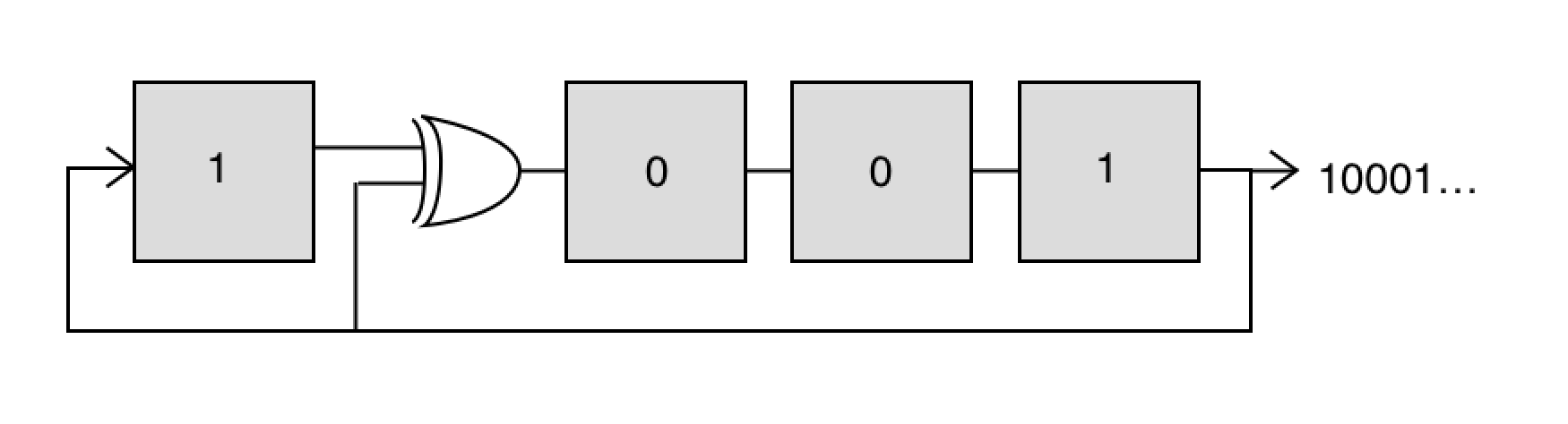
The specific type of PRBS that are used for generating EPD are the so called maximum length sequence (m-sequences) and these are typically generated using linear feedback shift register (LFSR). This is just a chain of flip-flops that is fed back on itself in a specific way to generate the PRBS of interest. To make this concrete, let’s consider a 4-bit LFSR implemented with 4 flip-flops and a xor gate as shown below. This circuit generates a repeating, length-15 series of bits: 100010011010111…
Now an important point is that these flip flips and gates tend to be relatively slow. However, serializers that convert multiple, parallel channels to a single, serial channel at a faster rate are available at quite high data rates (I’ve seen parts rated to above 50 Gbps). This suggests that a way to generate high speed PRBS is to generate multiple bits of the PRBS at a time and then combine them using a serializer. There are at least two approaches to this. One is simply to advance the sequence multiple bits at each clock. This turns out to be practical, although it requires some additional hardware. However, a more interesting, although not necessarily more practical approach, is generate alternating bits in parallel.
This second approach relies on an interesting property of these m-sequences: if one takes every other element of the sequence (this is referred to as decimation by twos), the result is a shifted sequence of the original sequence:
100010011010111100010011010111… ➡ 101011110001001…
100010011010111100010011010111… ➡ 000100110101111…
Examining these two sequences, we see that that both of the resulting sequences are just shifted versions of our original sequence, with the second sequence shifted 7 bits further than the first. With this result in hand, it’s clear that we can generate our sequence at twice the base rate if we combine two LFSR that are shifted by 7 bits with respect to each other.
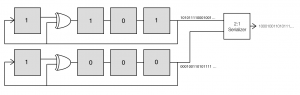
What’s particularly interesting about this is that the circuits to create the two sequences which we feed to the serializer are identical to the original LFSR except that they are initialized to different values. Furthermore, this trick can be extended to combining 4 shifted sequences using a 4:1 MUX by taking every fourth element of the original m-sequence to get shifted versions.
100010011010111100010011010111… ➡ 111100010011010…
100010011010111100010011010111… ➡ 000100110101111…
100010011010111100010011010111… ➡ 001101011110001…
100010011010111100010011010111… ➡ 010111100010011…
In fact, for longer sequences, one can take every 2nth element and always get a shifted version of the original sequence. For example, for a 10 bit LFSR, which can generate a 210-1 or 1023 bit PRBS, we could generate the sequence up to 512 bits at time using this scheme. A more realistic case would probably involve generating the sequence 64 bits at a time (this is the width of the serializers on some FPGAs). However, and this is where the possible impracticality comes in, one would need 640 flip flops as opposed to 10 flip flops for the base LFSR.
This might be acceptable in a pinch, but there is another approach that typically requires less resources. The figure shown below advances the PRBS two time steps for each clock cycle, where the two output bits can be read from the output of the two rightmost flip-flops.
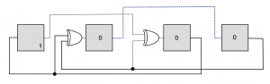
This has the same effect as the two parallel PRBS generators show above, but saves four flip flops. However, things get more complicated when generating a larger number of bits. In that case the signal needs to propagate through multiple xor gates at each clock, possibly slowing the maximum achievable data rate.
Despite the extra resources this takes up, this is an interesting way of exploiting the properties of m-sequences to generate PRBS at faster rates. It may slightly outperform the serial implementation when generating large number of bits at a time, so could be useful for generating very high rate signals. (A hybrid approach could also be envisioned where both techniques are used to reduce resources while preserving the maximum rate; interesting, but a topic for another day.)
NumPy on PyPy with a side of Psymeric
I’ve been playing around with PyPy lately (more on that later) and decided I’d take a look to see how the NumPy implementation on PyPy (NumPyPy[1]) is coming along. NumPyPy is potentially very interesting. Because the JIT can remove most of the Python overhead, more of the code can be moved to the Python level. This in turn opens up all sorts of interesting avenues for optimization, including doing the things that Numexpr does, only better. Therefore, I was very exciting when I saw this post from 2012, describing how NumPyPy was running “relatively real-world” examples over twice as fast as standard NumPy.
I downloaded and installed the NumPyPy code from https://bitbucket.org/pypy/numpy. This went smoothly except I had to spend a bit of time messing with permissions. I’m not sure if this was something I did on my end, or if the permissions of the source are odd. In either event, installation was pretty easy. I first tested the speed of NumPyPy using the micro-optimization code from last week – this was my first indication that this wasn’t going to be as impressive as I’d hoped. NumPyPy was over 10⨉ slower than standard NumPy when running this code!
I did some more digging around and found an email chain that described how the NumPyPy developers are focusing on completeness before speed. That’s understandable, but certainly isn’t as exciting as a very fast, if incomplete, version of NumPy.
I tried another, very simple, example, using timeit; in this case standard NumPy was about 7× faster than NumPyPy:
$ python -m timeit -s "import numpy as np; a = np.arange(100000.0); b=a*7"  "x = a + b"
10000 loops, best of 3: 71.3 usec per loop
$ pypy-2.3.1-osx64/bin/pypy -m timeit -s "import numpy as np; a = np.arange(100000.0); b=a*7" "x = a + b" 1000 loops, best of 3: 953 usec per loop
Just for fun, I dusted off Psymeric.py, a very old replacement for Numeric.array that I wrote to see what kind of performance I could get using Psyco plus Python. There is a copy of Psymeric hosted at https://bitbucket.org/dblank/pure-numpy/src, although I had to tweak that version slightly to ignore Psyco and run under both Python 2 and 3. Running the equivalent problem with Psymeric using both CPython and PyPy gives an interesting result:
python -m timeit -s "import psymeric as ps; a = ps.Array(range(100000), ps.Float64); b=a*7"  "x = a + b"
10 loops, best of 3: 30.7 msec per loop
pypy-2.3.1-osx64/bin/pypy -m timeit -s "import psymeric as ps; a = ps.Array(range(100000), ps.Float64); b=a*7" "x = a + b" 1000 loops, best of 3: 510 usec per loop
Running with CPython this is, predictably, pretty terrible (note the units are ms in this case versus µs in the other cases). However, when run with PyPy, this actually faster than NumPyPy. Keep in mind that Psymeric is pure Python and we are just relying on PyPy’s JIT to speed it up.
These results made me suspect that NumPyPy was also written in Python, but that appears to not be quite right. It appears that the core of NumPyPy is written in the RPython, the same subset of Python the PyPy itself is written in. This allows the core to be translated into C. However, as I understand it, in order for this to work, the core needs to be part of PyPy proper, not a separate module. And that appears in fact that is the case: the core parts of numpy are contained in the module _numpy defined in the PyPy source directory micronumpy and they are imported by the NumPyPy package, which is installed separately. If all that sounds wishy-washy, it’s because I’m still very unsure on how this is working, but this is my best guess at the moment.
This puts NumPyPy in an odd position. One of main attractions of PyPy from my perspective is that it’s quite fast. However, NumPyPy is still too slow for most of the applications I’m interested in. From comments on the mailing list, it sounds like their funding sources for NumPy are more interested in completeness than speed, so the speed situation may not improve soon. I should put my time where my mouth is and figure out how to contribute to the project, but I’m not sure if I’ll have the spare cycles soon.
[1] This was a name used for NumPy on PyPy for a while. I’m not sure if it’s still considered legit, but I can’t go around writing “NumPy on PyPy” over and over.