Let’s suppose I wanted to compute the sine of one of the angles of a right triangle given the length of two of its sides (don’t ask me why, that’s just the first example that popped into my head). In Python, I might start with a function like so:
def sin(x, y):
 return y / np.sqrt(x**2 + y**2)
Now suppose I want to calculate a whole lot of sine values? My first instinct is always to use NumPy. In this case, all I need to do is pass sin a pair of arrays instead of a pair of Python floats. If the resulting performance is good enough, we are done. If not, things get more complicated. There are several tools for speeding up this type of numerical code such as Cython, Weave, Numexpr, etc. I’ll discuss Numexpr in a bit, but first let’s see if there’s anything we can do to speed up the above function using Numpy itself.
The first step, of course, is to quantify the performance of our initial function. For this we throw together some simple benchmark code:
def make_x_y(n):
 return (np.random.random([n]),
         np.random.random([n]) + 1.0)

def test_timing(func, sizes, repeats=10):
 n_max = max(sizes)
 for n in sizes:
   x, y = make_x_y(n)
   t = 1e99
   for i in range(repeats):
     t0 = time.time()
     func(x,y)
     t1 = time.time()
     t = min(t, t1-t0)
   print("{0:e} ns per element: {1}".format(n, 1e9*t/n))
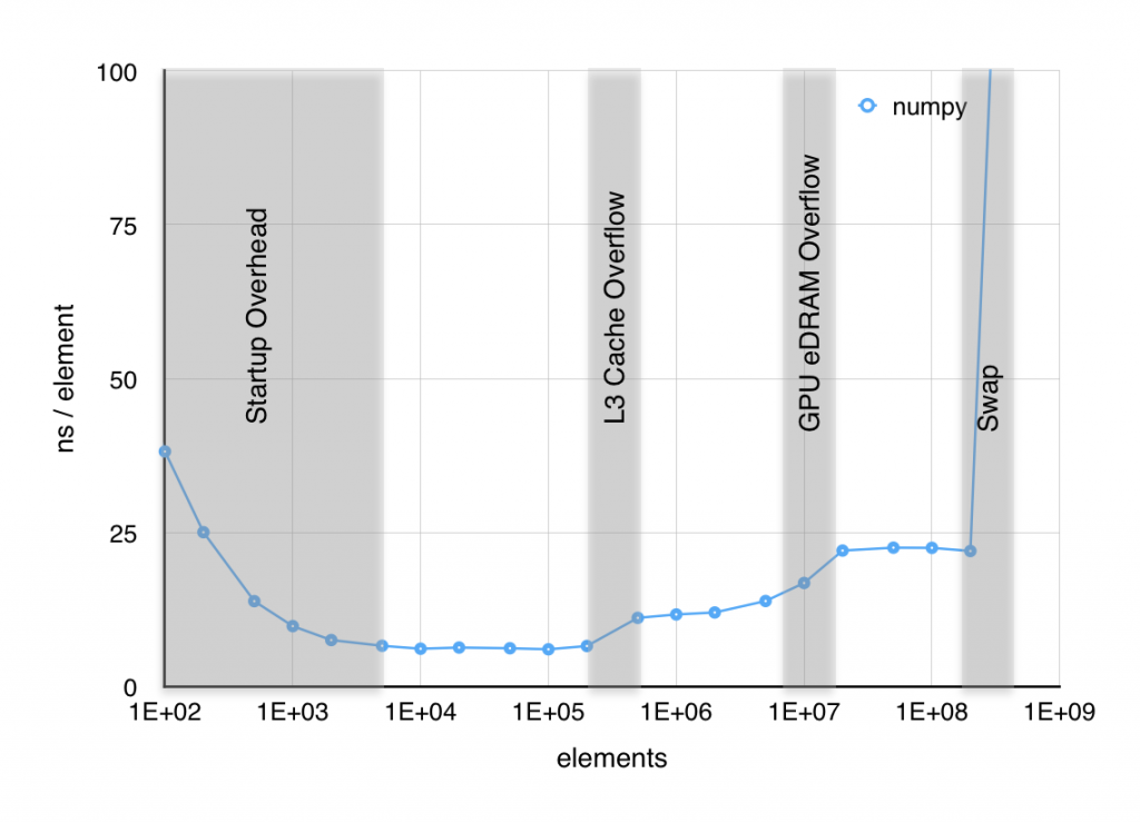
When I plot the time per element it takes to execute sin, several things are apparent. First, below about 103 elements, the result is dominated by setup overhead. Second, near both 106 and 107 elements, the time per element jumps significantly. Finally above 2×10⁹ elements, RAM starts to swap out to SSD and performance craters. The jump at 106 elements was easy to associate with the 6 MiB L3 cache starting to overflow, but the jump 107 was puzzling since, as far as I knew, the Haswell CPU in my macbook doesn’t have an L4 cache. However, I found out with a little digging, that some of the Haswell CPUs, including mine, have 128 MiB of GPU eDRAM that functions as a joint cache for the GPU and CPU. The overflow of what is effectively an L4 cache is likely the source of this second jump in time per element.

It is clear that part of our optimization effort should be directed to reducing these memory bottlenecks. I’ll show two approaches to this, the first using in-place operations and the second using a technique known as blocking. The first, in-place operations, takes advantage of the somewhat obscure out argument that most NumPy functions have as shown below. This significantly reduces the allocations of temporary arrays and thus should reduce both allocation overhead and the memory bottlenecks.
def sin_inplace(x, y):
 temp1 = np.empty_like(x)
 temp2 = np.empty_like(y)
 np.multiply(x, x, out=temp1)
 np.multiply(y, y, out=temp2)
 np.add(temp1, temp2, out=temp1)
 np.sqrt(temp1, out=temp1)
 np.divide(y, temp1, out=temp1)
 return temp1
The second approach is to break the calculation into smaller chunks so as not to overwhelm the cache. This is referred to as blocking although I sometimes still refer to it as chunking for obvious reasons.
CHUNK_SIZE = 4096
def sin_blocks(x, y):
 [n] = x.shape
 result = np.empty_like(x)
 for i in range(0, n, CHUNK_SIZE):
   x1 = x[i:i+CHUNK_SIZE]
   y1 = y[i:i+CHUNK_SIZE]
   result[i:i+CHUNK_SIZE] = y1 / np.sqrt(x1**2 + y1**2)
 return result
Finally, these approaches can be combined:
def sin_both(x, y):
 result = np.empty_like(x)
 [n] = x.shape
 buffer_size = min(CHUNK_SIZE, n)
 tmp_base = np.empty([buffer_size])
 for i in range(0, n, CHUNK_SIZE):
   x1 = x[i:i+CHUNK_SIZE]
   y1 = y[i:i+CHUNK_SIZE]
   [n1] = x1.shape
   tmp = tmp_base[:n1]
   r = result[i:i+CHUNK_SIZE]
   np.multiply(x1, x1, tmp)
   np.multiply(y1, y1, r)
   np.add(tmp, r, r)
   np.sqrt(r, r)
   np.divide(y1, r, r)
 return result
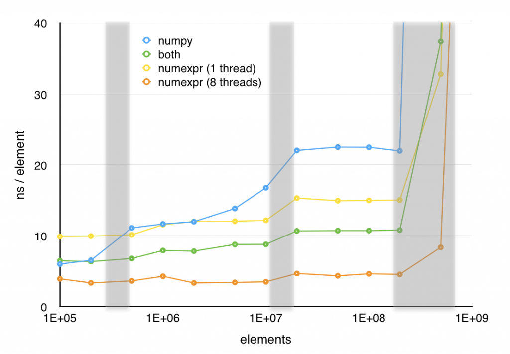
So far, I have taken a simple, clear function and turned it into three successively more incomprehensible ones. However, these new versions have one redeeming feature; as shown in the next plot, all three of these optimizations increase performance significantly. The in-place version is over 40% faster above 2×10⁶ elements and the other two versions offer even greater speedups (at least for large element counts) in exchange for their lack of readability.

These techniques might be useful in a situation where you need to squeeze a little more performance out of a specific bit of code, although I would recommend using them sparingly. Remember:
premature optimization is the root of all evil – Knuth
There are other approaches to speeding up Python and as promised, I’ll now say a bit about Numexpr. Internally, Numexpr automagically applies the blocking techniques discussed above to something that looks a lot like a NumPy expression. The most impressive part of Numexpr is not necessarily the speedup it delivers, but how clean the interface is:
import numexpr as ne
def sin_numexpr(x, y):
 return ne.evaluate("y / sqrt(x**2 + y**2)")
This takes the quoted expression, parses it, converts to byte code and then uses a specialized interpreter to perform the operation in chunks to improve performance. I would like to go into more detail on this, but this post is getting too long as it is and, more importantly, I haven’t looked at the internals of Numexpr in quite a while. One interesting, but superficial thing to notice though is that there is some sys._getframe() trickery going on here that allows evaluate to know the values of x and y without having them passed in.
Numexpr offers significant improvement in speed with very little loss of readability. Although, in this case the hand optimized code still performs better in the single threaded case, Numexpr does a good job of taking advantage of multiple cores and with 8 threads enabled, Numexpr handily outperforms the hand optimized code.
Numexpr is limited primarily to vector operations, although It does have some limited support for the sum and product reduction operations. It supports most of the vector operations one would consider a core part of NumPy including where, which can be leveraged to compute some expressions that would normally require a conditional. I refer you to the manual for the full list of supported expressions. While Numexpr has it’s limitations, it’s a fairly painless way to speed up certain classes of expressions in NumPy.
Next week: perhaps something about RPython? Or perhaps something simpler as this entry took longer than I’d planned.

